USD/JPY Pred Modeling ipynb

from alpha_vantage.timeseries import TimeSeries
import pandas as pd
import matplotlib.pyplot as plt
from sklearn.linear_model import Ridge  # Using Ridge regression
from sklearn.model_selection import train_test_split, GridSearchCV
from sklearn.metrics import mean_squared_error, r2_score
from sklearn.preprocessing import StandardScaler  # Standardization
import numpy as np

"""
Script to create a predictive model for USD/JPY

This script fetches daily USD/JPY data from the Alpha Vantage API
and builds a model using linear multiple regression to predict the next day's closing price.

The model is built using data over the following periods:
- 1 day
- 10 days
- 100 days
- 1000 days

Each model's performance is evaluated using RMSE and R^2.
"""

# --- Settings ---
api_key = "XXXXXX"
window_size_10d = 10
window_size_100d = 100
window_size_1000d = 1000  # Setting for 1000-day window

# --- Data Retrieval ---
print("---------- Starting data retrieval ----------")
ts = TimeSeries(key=api_key, output_format='pandas')
data, meta_data = ts.get_daily(symbol='USDJPY', outputsize='full')

from __future__ import print_function
print(data)
print("---------- Data retrieval complete ----------")

# --- Data Preprocessing ---
print("---------- Starting data preprocessing ----------")
data = data.rename(columns={
    '1. open': 'open',
    '2. high': 'high',
    '3. low': 'low',
    '4. close': 'close',
    '5. volume': 'volume'
})
data.index = pd.to_datetime(data.index)
data = data.sort_index(ascending=True)

# Feature Engineering
data['price_change'] = data['close'].diff()
data['high_low_diff'] = data['high'] - data['low']  # Difference between high and low
data['close_open_diff'] = data['close'] - data['open']  # Difference between close and open
data['volume_change'] = data['volume'].diff()  # Change in volume

# --- Moving Average Calculation ---
data['ma_short'] = data['close'].rolling(window=5).mean()  # Short-term MA (5 days)
data['ma_long'] = data['close'].rolling(window=25).mean()  # Long-term MA (25 days)

# --- RSI Calculation ---
delta = data['close'].diff()
gain = delta.where(delta > 0, 0)
loss = -delta.where(delta < 0, 0)
avg_gain = gain.rolling(window=14).mean()
avg_loss = loss.rolling(window=14).mean()
rs = avg_gain / avg_loss
data['rsi'] = 100 - (100 / (1 + rs))

# --- MACD Calculation ---
data['ema_short'] = data['close'].ewm(span=12).mean()  # 12-day EMA
data['ema_long'] = data['close'].ewm(span=26).mean()   # 26-day EMA
data['macd'] = data['ema_short'] - data['ema_long']
data['macd_signal'] = data['macd'].ewm(span=9).mean()  # Signal line

# --- Bollinger Bands Calculation ---
data['std'] = data['close'].rolling(window=20).std()  # 20-day standard deviation
data['upper_band'] = data['ma_short'] + 2 * data['std']  # Upper band
data['lower_band'] = data['ma_short'] - 2 * data['std']  # Lower band

# Handling missing values
data = data.dropna()

print("---------- Data preprocessing complete ----------")
# Display start and end date of data
print(f"Start date of data: {data.index[0]}")
print(f"End date of data: {data.index[-1]}")

# --- Model Building and Evaluation ---
def create_and_evaluate_model(data, window_size, model_name):
    print(f"---------- Starting {model_name} model processing ----------")
    X = data[['open', 'high', 'low', 'close', 'volume', 'price_change',
              'high_low_diff', 'close_open_diff', 'volume_change',
              'ma_short', 'ma_long', 'rsi', 'macd', 'macd_signal',
              'upper_band', 'lower_band']].values[:-1]
    y = data['close'].values[1:]  # Next day's close price

    X = X[window_size:]
    y = y[window_size:]

    X_train, X_test, y_train, y_test = train_test_split(X, y, test_size=0.2, random_state=42)

    # Standardization
    scaler = StandardScaler()
    X_train = scaler.fit_transform(X_train)
    X_test = scaler.transform(X_test)

    # Ridge regression model and grid search
    model = Ridge()
    param_grid = {'alpha': [0.01, 0.1, 1, 10, 100]}  # Regularization parameters
    grid_search = GridSearchCV(model, param_grid, cv=5, scoring='neg_mean_squared_error')
    grid_search.fit(X_train, y_train)

    best_model = grid_search.best_estimator_
    y_pred = best_model.predict(X_test)

    rmse = np.sqrt(mean_squared_error(y_test, y_pred))
    r2 = r2_score(y_test, y_pred)

    print(f"Best parameters ({model_name}): ", grid_search.best_params_)
    print(f"RMSE ({model_name}): {rmse:.4f}")
    print(f"R^2 ({model_name}): {r2:.4f}")
    print(f"---------- {model_name} model processing complete ----------")

    return best_model, scaler  # Return best model and scaler

# Evaluate models for each time window
model_1d, scaler_1d = create_and_evaluate_model(data, 1, "1-day")
model_10d, scaler_10d = create_and_evaluate_model(data, 10, "10-day")
model_100d, scaler_100d = create_and_evaluate_model(data, 100, "100-day")
model_1000d, scaler_1000d = create_and_evaluate_model(data, 1000, "1000-day")

# Get the latest data
latest_data = data.iloc[-1]  # Latest 1-day data

# Prepare features for prediction using each model
features = latest_data[['open', 'high', 'low', 'close', 'volume', 'price_change',
                        'high_low_diff', 'close_open_diff', 'volume_change',
                        'ma_short', 'ma_long', 'rsi', 'macd', 'macd_signal',
                        'upper_band', 'lower_band']].values.reshape(1, -1)

# Get prediction from 1-day model
prediction_1d = model_1d.predict(scaler_1d.transform(features))[0]

# Example: Using the 10-day model
latest_data = data.iloc[-window_size_10d:]  # Get the latest 10-day data

features = []
for i in range(len(latest_data) - 1):
    features.append(latest_data[['open', 'high', 'low', 'close', 'volume', 'price_change',
                        'high_low_diff', 'close_open_diff', 'volume_change',
                        'ma_short', 'ma_long', 'rsi', 'macd', 'macd_signal',
                        'upper_band', 'lower_band']].iloc[i].values)
features = np.array(features)

# Predict using the last day's features
prediction_10d = model_10d.predict(scaler_10d.transform(features[-1].reshape(1, -1)))[0]

# 100-day model
latest_data_100d = data.iloc[-window_size_100d:]  # Get the latest 100-day data

features_100d = []
for i in range(len(latest_data_100d) - 1):
    features_100d.append(latest_data_100d[['open', 'high', 'low', 'close', 'volume', 'price_change',
                        'high_low_diff', 'close_open_diff', 'volume_change',
                        'ma_short', 'ma_long', 'rsi', 'macd', 'macd_signal',
                        'upper_band', 'lower_band']].iloc[i].values)

features_100d = np.array(features_100d)

prediction_100d = model_100d.predict(scaler_100d.transform(features_100d[-1].reshape(1, -1)))[0]

# 1000-day model
latest_data_1000d = data.iloc[-window_size_1000d:]  # Get the latest 1000-day data

features_1000d = []
for i in range(len(latest_data_1000d) - 1):
    features_1000d.append(latest_data_1000d[['open', 'high', 'low', 'close', 'volume', 'price_change',
                        'high_low_diff', 'close_open_diff', 'volume_change',
                        'ma_short', 'ma_long', 'rsi', 'macd', 'macd_signal',
                        'upper_band', 'lower_band']].iloc[i].values)

features_1000d = np.array(features_1000d)

prediction_1000d = model_1000d.predict(scaler_1000d.transform(features_1000d[-1].reshape(1, -1)))[0]

# Get today's exchange rate
today_close = data['close'].iloc[-1]

# Print predictions
print("Today's Exchange Rate:")
print(f"Closing Price: {today_close:.4f}")
print("------------------")
print(f"1-day Model Prediction: {prediction_1d:.4f}")
print(f"10-day Model Prediction: {prediction_10d:.4f}")
print(f"100-day Model Prediction: {prediction_100d:.4f}")
print(f"1000-day Model Prediction: {prediction_1000d:.4f}")

# Calculate average prediction (example)
average_prediction = (prediction_1d + prediction_10d + prediction_100d + prediction_1000d) / 4
print("------------------")
print(f"Average Predicted Closing Price: {average_prediction:.4f}")

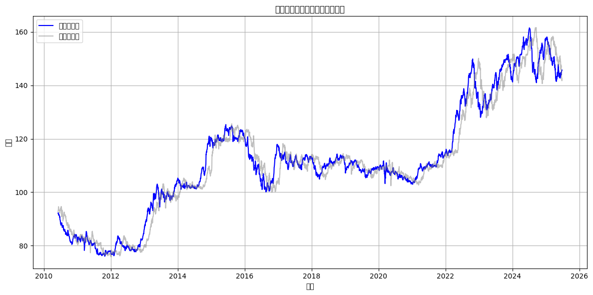
plt.figure(figsize=(12, 6))
plt.plot(dates, average_predictions, label="Average Prediction", color='blue')
plt.plot(dates, data['close'].iloc[start_index: start_index + len(dates)], label="Actual Closing Price", color='gray', alpha=0.5)
plt.title("Trend of Average Predicted Prices by Model")
plt.xlabel("Date")
plt.ylabel("Price")
plt.legend()
plt.grid(True)
plt.tight_layout()
plt.show()