Three-value classification(USDJPY) – Preparation, Learning, Importances

# import libraries
import pandas as pd
import numpy as np
import talib as ta
from sklearn.model_selection import train_test_split
from sklearn.ensemble import RandomForestClassifier
from sklearn.metrics import accuracy_score, precision_score, recall_score, confusion_matrix
import optuna
import matplotlib.pyplot as plt
import seaborn as sns

# Check the shape
print(df0.shape)

# Check the data
summary = df0.describe()
print(summary)

# # Display information about the DataFrame
df0.info()

df0["Date"] = pd.to_datetime(df0["Date"])

# Get the oldest and latest dates
oldest_date = df0["Date"].min()
latest_date = df0["Date"].max()

print("Oldest Date:", oldest_date)
print("Latest Date:", latest_date)

df0["Date"] = pd.to_datetime(df0["Date"])

# Get the oldest and latest dates
oldest_date = df0["Date"].min()
latest_date = df0["Date"].max()

print("Oldest Date:", oldest_date)
print("Latest Date:", latest_date)

# Load and clean the data for df1
df1 = pd.read_csv("")
df1["Date"] = pd.to_datetime(df1["Date"], format="%m/%d/%Y")  # Specify the correct date format

# Concatenate DataFrames
df = pd.concat([df0, df1])

# Calculate oldest and latest dates
oldest_date = df["Date"].min()
latest_date = df["Date"].max()

print("Oldest Date:", oldest_date)
print("Latest Date:", latest_date)

print(df.shape)

df.info()

# Drop the "Vol." column from df
df = df.drop("Vol.", axis=1)

# Check the shape of df after dropping the column
print("Shape of df after dropping 'Vol.' column:", df.shape)

# Identify columns with all null values
null_columns = df.columns[df.isnull().all()]

# Drop columns with all null values
df = df.drop(columns=null_columns)

# Check the shape of df after dropping null columns
print("Shape of df after dropping null columns:", df.shape)

# print the unique column names in df
print("Unique column names in df:", df.columns.tolist())

#All subsequent calculations use the closing rate
close = np.array(df["Price"])

#Create an empty dataframe to contain features
df_feature = pd.DataFrame(index=range(len(df)),columns=["SMA5/current", "SMA20/current","RSI","MACD","BBANDS+2σ","BBANDS-2σ"])

#Ccalculate technical indicators (features used in this training) using talib and put in df_feature

#Simple moving average uses the ratio of the simple moving average to the closing price of the day as the feature value
df_feature["SMA5/current"]= ta.SMA(close, timeperiod=5) / close
df_feature["SMA20/current"]= ta.SMA(close, timeperiod=20) / close

#RSI
df_feature["RSI"] = ta.RSI(close, timeperiod=14)

#MACD
df_feature["MACD"], _ , _= ta.MACD(close, fastperiod=12, slowperiod=26, signalperiod=9)

#Bollinger bands
upper, middle, lower = ta.BBANDS(close, timeperiod=20, nbdevup=3, nbdevdn=3)
df_feature["BBANDS+2σ"] = upper / close
df_feature["BBANDS-2σ"] = lower / close

df["the day before_float"] = df["Change %"].apply(lambda x: float(x.replace("%", "")))

#How to categorize the % of previous day. Divide as much as possible so that the sample of each class is equal
def classify(x):
    if x <= -0.2:
        return 'down'
    elif -0.2 < x < 0.2:
        return 'even'
    elif 0.2 <= x:
        return 'up'


df["the day before_classified"] = df["the day before_float"].apply(lambda x: classify(x))

#Shift the data you want to teach by one day (you know what I mean)
df_y = df["the day before_classified"].shift()

# Reset the index of df0_y to ensure uniqueness
df_y = df_y.reset_index(drop=True)

# Concatenate df0_feature and df0_y with reset index
df_xy = pd.concat([df_feature, df_y], axis=1)
df_xy = df_xy.dropna(how="any")

# print("Shape of df_xy:", df_xy.shape)
print("Number of samples in df_xy:", len(df_xy))

X_train, X_test, Y_train, Y_test = train_test_split(
    df_xy[["SMA5/current", "SMA20/current", "RSI", "MACD", "BBANDS+2σ", "BBANDS-2σ"]],
    df_xy["the day before_classified"],
    train_size=0.8,
    random_state=42
)

print("Shape of X_train:", X_train.shape)
print("Shape of X_test:", X_test.shape)
print("Shape of Y_train:", Y_train.shape)
print("Shape of Y_test:", Y_test.shape)

X_train, X_test, Y_train, Y_test = train_test_split(df_xy[["SMA5/current", "SMA20/current","RSI","MACD","BBANDS+2σ","BBANDS-2σ"]],df_xy["前日比_classified"], train_size=0.8)

def objective(trial):
    min_samples_split = trial.suggest_int("min_samples_split", 2,16)
    max_leaf_nodes = int(trial.suggest_discrete_uniform("max_leaf_nodes", 4,64,4))
    criterion = trial.suggest_categorical("criterion", ["gini", "entropy"])
    n_estimators = int(trial.suggest_discrete_uniform("n_estimators", 50,500,50))
    max_depth = trial.suggest_int("max_depth", 3,10)
    clf = RandomForestClassifier(random_state=1, n_estimators = n_estimators, max_leaf_nodes = max_leaf_nodes, max_depth=max_depth, max_features=None,criterion=criterion,min_samples_split=min_samples_split)
    clf.fit(X_train, Y_train)
    return 1 - accuracy_score(Y_test, clf.predict(X_test))

study = optuna.create_study()
study.optimize(objective, n_trials=100)

print(1-study.best_value)
print(study.best_params)

# Create and train a RandomForestClassifier
model = RandomForestClassifier()
model.fit(X_train, Y_train)

# Predict the target values for the test data
Y_pred = model.predict(X_test)

# Calculate the accuracy, precision, recall
accuracy = accuracy_score(Y_test, Y_pred)
precision = precision_score(Y_test, Y_pred, average='weighted')  # You can also use 'macro' or 'micro'
recall = recall_score(Y_test, Y_pred, average='weighted')  # You can also use 'macro' or 'micro'

print("Accuracy:", accuracy)
print("Precision:", precision)
print("Recall:", recall)

#　Create and train a RandomForestClassifier
model = RandomForestClassifier(n_estimators=100, random_state=1)
model.fit(X_train, Y_train)

# Get feature importances
feature_importances = model.feature_importances_

# Create a DataFrame to associate features with their importances
importance_df = pd.DataFrame({"Feature": X_train.columns, "Importance": feature_importances})
importance_df = importance_df.sort_values(by="Importance", ascending=False)

# Print or visualize the feature importances
print(importance_df)

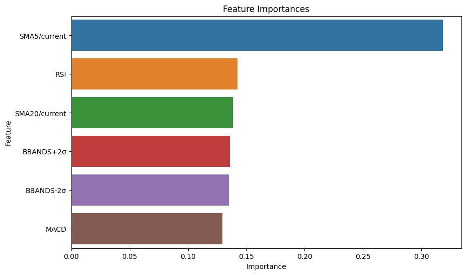
plt.figure(figsize=(10, 6))
sns.barplot(x="Importance", y="Feature", data=importance_df)
plt.title("Feature Importances")
plt.xlabel("Importance")
plt.ylabel("Feature")
plt.show()